Please, read the file, readme.txt, that came with SAR Image Processor.
Because this is a single page manual that contains many images, it may take a long time to download. The advantage to having everything on one page is that you can use your browser's Find function to serve as an index. To save time with future viewing of this manual, you should save this web page as an MHT file on their hard disk. Then, you can refer to this MHT file and need only occasionally check this web page for changes.
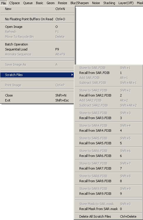
SAR is unusual because it uses a 32 bit/channel floating point buffer. There is no traditional undo. There are nine scratch files for storing intermediate results. Use Shift + 1-9 (Number keys) to store and 1-9 to recall.
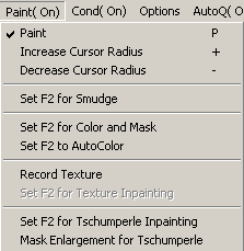
Some operations must be applied with the F2 or F3 key, in which case, the operations are automatically loaded by clicking a menu item. When possible, pressing F2 will reverse the effect F3 and vice versa. Some operations can be painted, in which case, the right/middle mouse buttons have the same operations as F2/F3. Some operations are not automatically loaded into F2/F3 but normally take effect immediately after the menu item is clicked. Usually these operations, e.g., Geom>Horizontal Flip, can be loaded to the F2 key by holding the Control key down before clicking on the menu item. Some people have difficulty with this probably because the Control key must be held down and not released BEFORE the main window loses focus to the menu. A mnemonic name for the loaded operation is displayed as the last item on the menu bar as shown in the following figure:

Observe that loaded operations are queued and displayed in a pop down menu. This menu functions as a programmable tool bar, but is better because it doesn't obstruct anything and uses mnemonic words instead of icons. Also, the queued operations can be scrolled with the comma, period (< >) keys. These queued operations persist between closing and reopening SAR because they are saved in the sar.ini file. When parameters settings need to be changed, pressing F4 will bring up the dialog box for the active operation. I suggest that you stop here and practice manipulating these features.
In batch processing (File>Batch Operation), the active F2 operation, but not the F3 operation, is directly applied to multiple files. However, an F3 operation can be indirectly applied by incorporating it into an "action" which is itself an F2 operation. Only operations applied with F2 and F3 can be recorded into an action. You will need a dummy image to record an action. Use Prog>Record Program to start. Then up to 32 operations, applied by pressing F2 or F3, can be recorded, along with their parameter settings. After unchecking Record Program, a dialog box will appear showing a list of recorded operations. Then "RunProg" will appear as the loaded operation.
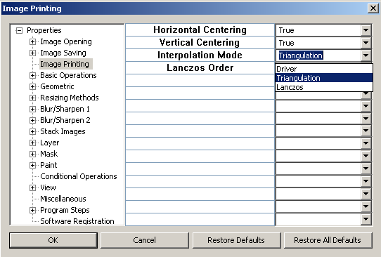
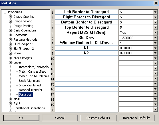
Regarding the Properties Dialog Box,

all properties set with this dialog are saved in the file, sar.ini, when SAR closes and read when the SAR opens. Most parameters have value limits for entry. To see whether your entry was accepted, click on another tree item and then back to the original. If your entry was not accepted, the previous value will be displayed. The tree structure on the left corresponds very roughly to items as they appear on the menu bars. There is no outstanding need to navigate this tree because clicking on a menu item or pressing F4 automatically opens the dialog to the correct tree position. However, there are some settings that are only accessible from the tree, e.g., Properties>View>Background Grey Level. The dialog box can also be accessed by pressing the Q key.
Creates an additional window. It should be noted that, unlike some other software, SAR does not automatically open an image in a new window. In combination with synchronized scrolling, multiple windows are most useful for side by side comparison of similar images. Multiple windows share the same parameter settings and scratch files.
With this option checked, no floating point buffer will be created when an image file is read. The purpose of this is to conserve RAM for interpolation operations. With this option checked, SAR will not read or write file formats greater than 24 bit. Most operations, other than some resizing operations and printing, will be disabled without a floating point buffer. Also, it is sometimes possible to create images that are too large to save. (Microsoft code contained in the GDIPLUS.DLL is used for 24 bit files, so I blame Microsoft.)
SAR reads 24 and 48 bit integer and 96 bit floating point TIFF subformat. SAR normally reads 24 and 48 bit PNG. SAR reads two proprietary formats, FDIB and IFS, which may not be compatible with future versions.
Tip:
There is no outstanding need to use the Open Dialog box because
1. You can conveniently open a file into SAR from Windows Explorer.
2. Almost all SAR settings persist between opening and closing SAR. In particular, the F2/F3 operations persist.
3. SAR opens fast.
For me, a very annoying fault of Microsoft's Open/Save Dialog box under Windows XP is that display settings, e.g., View Thumbnails, do not persist between openings and closings. This anti-ergonomic nonsense is avoided by opening a file from Windows Explorer.
Select multiple files in dialog box by holding down the Ctrl key. The F2 programmed operation will be applied to each file and (*with two exceptions) saved. Overwriting can be avoided by attaching a suffix to every file name. During processing, the number of images is counted in the fifth pane of the status bar. The user can control the file buffer size by setting the parameter, Maximum Characters. A larger buffer size will be necessary to read a sufficiently large file list. If you encounter a failure, it may be easier to test the adequacy of a larger setting by using Sequential Load rather than Batch Operation, since this feature is shared.
*A processed image is not saved when F2 is programmed with Print or recorded actions ending with Print.
Initially, multiple selections are made from a dialog box by holding down the Ctrl key, after which, each time key F9 is pressed, a new file is loaded from that selection until the sequence is completed. You can back up by pressing Shift+F9. The sequence can be prematurely terminated by pressing Ctrl+F9, or holding down the Ctrl key before clicking menu item. The number of images is counted in the fifth pane of the status bar. If the sequence terminates prematurely, it is probably because the size of a buffer which holds file names was exceeded. To fix this problem, increase the buffer size by setting the shared Batch parameter, Maximum Characters. If you use this for a slideshow instead of processing, it is better that File>No Floating Point Buffer On Read be checked because files will load faster.
Use this after Sequential Load above to automatically display the images at a specified time interval in between. For example, with Irfanview, you can decompile an MPEG file into still frame BMP files. Using SAR's batch capability, you can retouch and enlarge these frames. Then you can use Animate Sequence for a better animated visual display than with the original MPEG. Again, it is better that File>No Floating Point Buffer On Read be checked because files will load faster.
There is no "Save" because it is generally bad practice to overwrite image files. This is particularly true with SAR because EXIF information is lost. Unlike with other programs, using "Save As," will not make the saved file the active file. Also, when closing SAR, there is no dialog box asking whether you want to save the image. Remember, a scratch file, e.g., saved with Shift + 1, stays on your hard disk when SAR closes. That is how you should save a work in progress. SAR's native format is the FDIB (*.fdib) file, which contain information about the color space, channel selection, and mask. FDIB is the only file type that can change the color space and channel settings when the file is opened.
There are five image file formats that have property settings:
These are nine FDIB files that are saved in the same directory that you installed sar.exe. Warning, these files are large and stay on your hard drive until you delete them! Use Shift + 1-9 to store and 1-9 to recall.
New with version 4.3, Key 0 is used to store masks. To load a mask with Shift+0, the current image must be of the same dimensions.
Attention users of older SAR versions! Key 0 was previously used to set pixel values to zero. That operation is now Shift+Z.
First, this dialog box appears:
followed by this
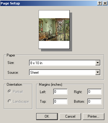
Important Note: The settings for the Page Setup Dialog (e.g., margin settings, paper size) and the Printer Properties Dialog (e.g., paper type) are not preserved when SAR closes. Whenever SAR opens, these settings will be the defaults which the user can set via the Windows OS. However, such settings, once made in SAR, will persist until SAR closes. Also, there is a "bug" under Windows ME (and probably 98 and 95), but not XP, in which a sufficiently large image may fail to show in the preview window of the Page Setup dialog box. This bug does not affect printing.
Automatic interpolation to optimum size for printing via Lanczos or Triangulation will usually result in better prints than using the interpolation built into the printer driver. However, for superior results, I recommend that images first be enlarged 4X by edge preserving methods.
Attention! Starting with SAR 4.2, a bug preventing printing with Canon printers has been corrected. (I discovered this bug the hard way, by buying a Canon printer.)

The color space selection is indicated in the second pane of the status bar
and check marks in the menu. The channel selections are
indicated in the third pane of the status bar and check marks in the
menu. For example, the above settings produce these  status
bar panes. When you check color spaces, you may be surprised that the
menu stays open so that you can make additional checkings. This is
an ergonomic feature of SAR. You can close the menu by
pressing F10 or clicking on the main window. Many, but not all,
operations are applied only to selected color spaces. In some cases this
allows some useless combinations, e.g. applying gamma transformation to H
channel of HSV space. The selection of channels can be
conveniently toggled on and off (between selecting
all channels) with menu item "Cond()" (F12), but it is likely
to accidentally leave this on so I made Cond(Off)
red so that I would notice.
status
bar panes. When you check color spaces, you may be surprised that the
menu stays open so that you can make additional checkings. This is
an ergonomic feature of SAR. You can close the menu by
pressing F10 or clicking on the main window. Many, but not all,
operations are applied only to selected color spaces. In some cases this
allows some useless combinations, e.g. applying gamma transformation to H
channel of HSV space. The selection of channels can be
conveniently toggled on and off (between selecting
all channels) with menu item "Cond()" (F12), but it is likely
to accidentally leave this on so I made Cond(Off)
red so that I would notice.
This is the default mode. SAR's RGB is similar to conventional RGB except intensity values less than zero and greater than 255, as well as non integral values, are allowed. As with all SAR color spaces, appropriate clipping and rounding to integer values is performed outside of the floating point buffer.
There are slightly different standards for YCbCr because the calculation is based on the characteristics of various phosphors use color television and monitors. SAR uses basically the same standard that JPEG, TIFF, and PNG uses. Interestingly, this is based on phosphors used in late 1950s' television.
Roughly speaking, brightness is represented by Y (Luminance) and color is represented by Cr and Cb. More specifically, Y = 0.2990*R + 0.5870*G + 0.1140*B where R, G, B are RGB channel values. Setting the Cr and Cb intensities of all pixels to zero will result in a grey scale (BW) image. Multiplying the Cr and Cb intensities by a number greater than one, e.g., 1.1, will increase the color saturation. The terms "roughly speaking" are used here because results will differ from those produced by other methods. This color space can be used with some interpolation methods to an advantage. Also, the Cr and Cb channels are often useful in conjunction with Mask>"Set F2, F3 to Mask by Color."
Similar to YCbCr, except Y = (R+G+B)/3.
H is the hue which varies cyclically from 0 to 360 degrees. Red is 0, green is 120 and blue is 240. S is color saturation and normally varies between 0 and 1. V, another measure of brightness, stands for "value" and simply represents the maximum R, G, an B value and therefore normally varies between 0 and 255. Again, the range for these numbers has been increased in the floating point buffer. The hue of a color of saturation zero (black, grey and white) has been arbitrarily defined as 0 (red). For that reason, do not use any operation on the S channel that will make previously zero values positive. Otherwise, white areas will become pink or red. Multiplication and Gamma are safe to us on the S channel. Do not use HSV with interpolation!
Similar to HSV, except I, intensity, represents the average of RGB values. Also, there are subtle differences between the H and S components of HSI and HSV. Do not use this with interpolation!
Adding two images in this color space produces a result identical to that of overlaying two transparencies of the images. White is completely transparent and black is completely opaque. If you want to add text to an image, just add a black and white text image.
Performs a gamma transformation with a gamma value that can be selected under Miscellaneous.
Performs RGB Gamma transformation before converting to YCbCr.
With "Cond( On)" on the menu bar, certain operations will only be applied to checked channels. When one of these menu items is clicked, the pop up menu will automatically reappear. Pressing the F10 key or clicking elsewhere, e.g., another menu item, will close the menu. Color space selections can also be made using keys, 1, 5, and 9. The selection status can also be read in the third pane of the status bar.
Makes orthogonal color channels that depend on the image. Currently, only experimental.
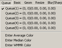
Displays and/or stores coordinate and/or color information for use with the following operations:
When only one point or color is involved, the checked queue color applies. When multiple or variable points or colors are involved, they are applied from the top of the queue. Coordinate and/or color information can be entered in three ways:
First, by left clicking on an image pixel and pressing the Enter key. This will place the pixel information on the top of the queue. Previously entered values are shifted downward.
Second, coordinate and color information can be manually edited from dialogs. Holding down the Shift while clicking on the menu item will bring up the coordinate dialog. Similarly, the Ctrl key will bring up the color dialog. Enter numbers separated by commas.
Third, the following three operations enter colors into the queue.
The average color for an image area is placed into the queue. Normally, this area applies to the entire image, but this can also be an unmasked area or a painted area. When this operation is applied by clicking on the menu, the menu will reappear so that you can examine the color at the top of the queue. You can close the menu by pressing F10 or just clicking elsewhere.
Similar to Enter Average Color. Average is replaced by median.
Similar to Enter Average Color. Average is replaced by wmmr.

Self explanatory. In RGB space, this can be used to adjust brightness.
Self explanatory. In RGB space, this is similar to contrast control.
This linearly changes the minimum while the luminance at 255 remains fixed.
Reshapes the histogram by exponentiation of intensity values. Roughly speaking, in RGB space, F2 darkens while increasing contrast and color saturation, F3 lightens the image while decreasing contrast and color saturation. In other color spaces, you need to study the effect.
Produces maximally flat histogram (subject to some constraints).
The following dialog box will appear:

after which, a graph similar to this will appear:
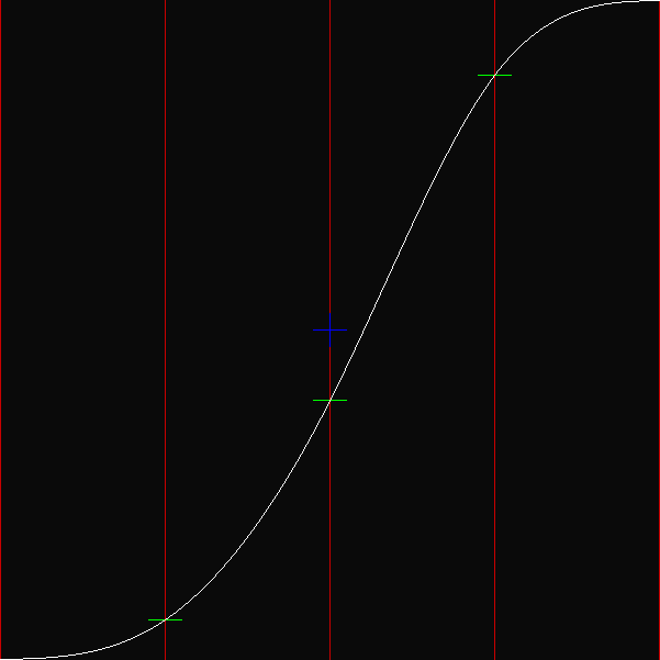
The middle "control points" are where the green horizontal line segments
intersect the faint red vertical lines. To shape the curve, move the
control points along the vertical faint red lines. To move a control
point, hold the left mouse button down while moving the mouse cursor on the
control point. While this is done, the mouse cursor will change from an
arrow to a hand. You can also move the end points, but it is recommended that
you don't. To use this curve to adjust image luminances, the curve must be
monotone increasing. Nonincreasing parts of the curve will be shown in
pink. You can also avoid nonincreasing parts by setting the fourth
parameter, Constrain Monotone Increasing, to True, but I find that this makes
adjustments more difficult.
The seventh parameter, Control Points Preset, sets the control points to the points of the selected function before you make adjustments. If you want to make further adjustments to a previously designed curve, this parameter should be set to None.
The control points (and their number, 6th parameter) plus the 1st, 2nd, 3rd and 5th parameters generate a lookup table that is used on the pixel luminances. The dimensions of the graph are always equal to the Number of Lookup Elements (5th parameter). The curve does not generally pass exactly through the control points. To increase/decrease the vertical distances of the curve from the control points, decrease/increase, the 3rd parameter, Weights for Middle Points. The graph image can be saved and processed like any other image, but you may first have to create a floating point buffer (Control+Y). After restoring the temporarily saved image by unchecking this menu item, apply the curve with F2 or its inverse with F3. Note that your custom curve can be saved by incorporating it into an action. This operation can be painted.
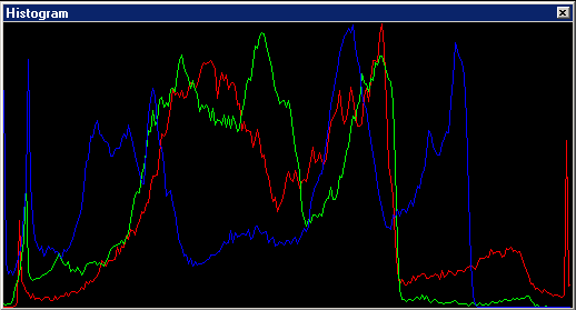
An image histogram is a graph with abscissa denoting pixel intensity and ordinate denoting the frequency of occurrence. The SAR histogram may differ from histograms of other programs in several ways. In SAR, clipped values are not shown. For example, in SAR, RGB values less than zero and greater than 255 do not appear, but, in other histograms, may appear as respective values, zero and 255. Adding/subtracting a positive constant from a color channel of an image will shift its histogram to the right/left. Multiplying/dividing a color channel by a constant greater than one will expand/contract the histogram about zero.
Also, the SAR histogram depends on color space selection. For example, in HSV mode, the H channel is shown in red, the S channel in green, and the V channel in blue.
Self explanatory. Color in checked queue is applied.
F2/F3 interpolates/extrapolates between the input image and a homogeneous image of the color specified in the checked queue element. By placing the median color of the image into the queue element, conventional contrast adjustment can be derived.
Sets pixel intensity values to zero.
Uses the top two queue coordinate and color entries to produce a linear variation of color.
Self explanatory in RGB space.
New with SAR 3.1! All image morphing is done with Lanczos3 interpolation! (Previous versions used bicubic.)
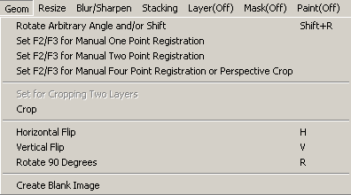
The image will be rotated about its center by any amount entered into the dialog box. Starting with v. 3.1, you can also shift by an arbitrary amount. The unknown portions of the rotated image will be filled with a reflection which often, especially for small angles, will provide plausible fiction. If you do not like these reflections, set the mask (press M key) before the rotation. Then, after rotation, reflected parts will be unmasked. These unmasked portions will be displayed as black, but do not directly affect the image. To make these portions actually black, press zero key.
If you load this operation into the F2 and F3 keys, pressing the F3 key will rotate and translate opposite to the amounts entered. The F2 and F3 keys will undo each others' effects, except there will be a small amount of blur/artifacts remaining from interpolation. You have the option of reducing these blur/artifacts with iterative refinement. Translation is after/before rotation for F2/F3, respectively.
Uses the checked coordinate in the Queue as the destination point. Recall that a point is entered into the Queue by left clicking on image point, followed by pressing Enter key. The source point is similarly recorded, but without pressing the Enter key. When the F2 key is pressed, the image will be translated so that the spot in the image marked by the source point is now at the destination point. The image will wrap around the canvas so that no portion of the original image is lost. The F3 key switches source and destination points and therefore can be used to undo the F2 operation.
Tips: Afterwards, fine one pixel adjustments can be made by using the Arrow keys with Ctrl key held down. When manually aligning an image in the top layer to an image in the bottom layer, it is useful to use Options>"Show Difference Between Layers," (press D key).
This operation uses the top two coordinates in queue as destination points. These points are entered by left clicking the mouse cursor followed by pressing the Enter key The source points are similarly produced but WITHOUT pressing the Enter key. The image will be translated, rotated, and resized so that the spots in the image marked as the source points are moved to the destination points by morphing the image. Similar to Rotation (see above) unknown portions of the image will be filled in with reflections and etc..
Similar to above, but uses two sets of four points as source and destination. With the Perspective Crop setting, the source points are those with the Enter key and the destination points are automatically the corners of the image.
When set and there is second layer of equal dimensions, Crop will be applied to both layers.
This allows selection of the area to be cropped by entering coordinates of the bottom left corner and dimensions of the selected area in a dialog box.
Also, this can be used as a fine adjustment to cropping with the mouse. With the right mouse button held down, moving the cursor over the image will produce a rectangle. (Paint must be off.) As the mouse is moved, the dimensions of the rectangle is displayed in the first pane of the status bar. Normally, upon releasing the right mouse button, the image is immediately cropped to that rectangle. However, if the Ctrl key is held down while the mouse button is released, there will be no immediate cropping and the rectangle will remain. Then, when Crop is used, the coordinates and dimensions of the rectangle will appear as default values in the dialog box which, then, may be edited.
Tip: Mouse crop large images by using F5 and F6 view options.
Self explanatory.
Self explanatory.
Self explanatory.
Self explanatory.
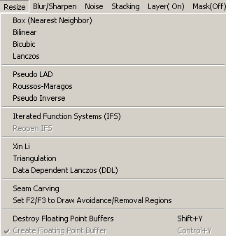
Attention! Some people claim that there should be gamma 2.2 correction for resizing. For example, see http://www.all-in-one.ee/~dersch/gamma/gamma.html and http://tech.slashdot.org/article.pl?sid=10/02/23/2317259. To do this in SAR, for methods without a "shortcut" parameter in the dialog box, select CSpace>RGB GammaX or CSpace>YCbCr GammaX before resizing. For methods with a "shortcut" parameter in the dialog box, select one of those color spaces in the dialog box (YCbCr GammaX is faster).
Most interpolation methods show a progress bar in the 6th pane of the status bar. Also, pressing Ctrl+Break key while the progress bar moves will terminate processing.
All of the linear methods can be used for both enlargement and reduction of images to arbitrary scale factors. The nonlinear methods can only be used for enlargement and directly only with integer scale factors and, in some cases, only with a power of 2, i.e., 2, 4, 8, etc. However, in some nonlinear cases, you can indirectly scale to noninteger scale factors. There are size limits and, in some cases, you have the option to increase the size limit at the cost of speed or quality. This is done by avoiding floating point buffers with either File>No Floating Point Buffers On Read or Resize>Destroy Floating Point Buffers. A rough rule of thumb is that, under Windows XP, the sum of input and output pixels is limited to 80 megapixels with floating point buffers, and 345 megapixels without floating point buffers. When you exceed the limit, you will get warning messages, but SAR should not crash. There are variances between different computers systems that I cannot fully explain. You also may run into trouble saving a very large image, in which case, you should try a different file format.
Also, remember that you can use small crops to quickly adjust parameter settings by trial and error for everything except IFS because, except for a small region near to the image border, input size does not affect quality. IFS is different because, all else equal, overall quality will improve with increasing size of the input image.
This Dialog Box controls the output dimensions:

"Precedence" values have the following effects:
Kernel Expansion for Reductions - Only affects reductions. Setting to True provides antialiasing.
Also, called "nearest neighbor," in enlargements, each pixel is represented by a square. In reductions, pixel outputs are obtained by simple averaging of pixels within nonoverlapping square areas. Enlargement results are visually unappealing, but useful for inspecting the results of other image processing operations. Box reductions are fairly descent looking. This is the only rescaling method offered here such that upscaling by integral scale factors, followed by downscaling to original size, gives a result exactly identical to the original image.
Bilinear is relatively useless for enlargements but it is sometimes useful for
size reductions because it produces no halos.
A standard method, but rarely is the user given access to an endemic parameter, called here "Bicubic Sharpening Factor." A value of -1 results in maximum sharpening and 0 results in least sharpening. A 4x4 window of input pixels is used to calculate each output pixel.
The user selected "order" parameter controls the effective size, in pixels, of the input window used to calculate an output pixel:
As order is increased, lines and edges in the output image become less jagged, but "ringing" around edges increases. Order 3 is best for most images. Note, any order between 2 and 64 can be entered.)
Lanczos 3 is most useful for size reductions because it produces sharper results with less jagged edges than other methods offered here, however, unlike box and bilinear, it produces halos.
This normally requires more RAM than most other methods and it is also fairly slow. For typical digicam images you will probably have to either destroy the floating point buffer (Shift+Y) or check File>No Floating Point on Read before loading an image file, in which case, the size of input plus output images should be limited to about 345 megapixels, but I don't guarantee it.
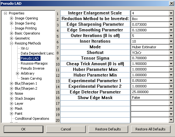
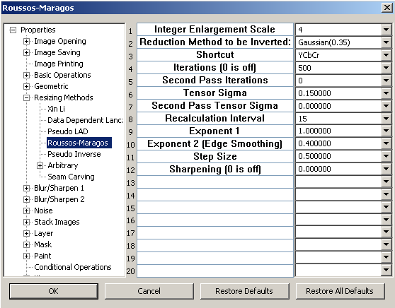
Referring to numbered parameters in above dialog box:

Refer to above dialog box. Pseudoinverse works only with integer scale factors. The resulting enlargement, when reduced back to original size by the method selected (1), will almost exactly match the original. The parameters of the next two lines, (2) and (3), can compensate for some sharpening or blurring. The "Inverse Sharpening Radius" is automatically scaled to the smaller image, e.g., "1" represents a radius of one pixel in the smaller image. This was to keep the settings independent of scale. Setting the last line to True will produce a reduction based on (1), (2) and (3) which can be used to match edge characteristics (halos, sharpness, etc.) of the image you want to enlarge. These settings are also used by SuperRez postprocessing. With proper settings, SuperRez will eliminate almost all edge jaggedness and halos while sharpening edges. The parameter "Based on Enlargement by" should be of slightly higher order than the method selected in (1). Using a small crop, you should determine the settings that work best for your image by trial and error. The wrong settings will probably give bad results.
SAR's implementation is similar to, but far from identical to Genuine Fractals (GF). To the best of my knowledge, SAR is the only program other than GF to offer IFS interpolation. Furthermore, unlike with GF, there is no attempt at file compression and SAR's IFS files can easily become very large.
Although IFS can be accessed as a one step process from the Resize menu, it can also be accessed as a two step process from the File menu; From the File menu an image is saved as an IFS file which can be opened at any time to a desired size. In the Resize menu, IFS has been combined into single step in which internally a temporary IFS file is saved and opened. Besides allowing unregistered users of SAR to test IFS, the single step allows batch processing.
Below are the IFS dialog boxes showing default values.

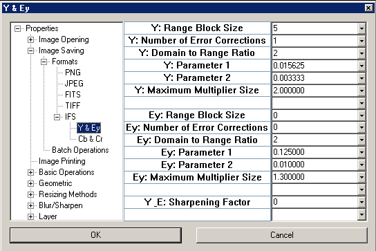
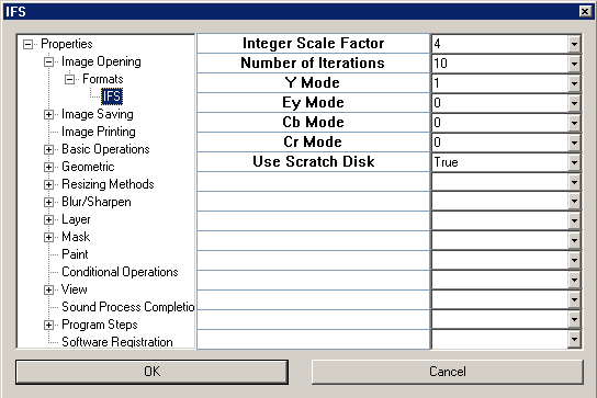
For IFS saving, there are many parameters to set, and they do have a strong influence on the results. There is one important thing to always bear in mind when using IFS; all else equal, the quality (PSNR) of the result will increase with the size of the input image. Also, all else equal, the time required for the "saving" operation will be proportional to the square of the area (megapixels) of the input image. For that reason, if you make certain settings for a large input image, IFS can take days to process. To make things easier, I have included a simplified dialog. With Use Custom Settings set to False, the custom save dialogs containing the actual IFS parameters will not appear. With the simplified dialog, the user should select the size and quality values that most closely represent the input image. The low quality setting was designed to sharpen blurry edges and obliterate noise, JPEG artifacts, and moire pattern at the expense of texture details. This setting should be considered a cosmetic effect, as it will lead to low PSNR values. I use this setting on images from my Epson 3100z digicam to obliterate moire pattern and sharpen the edges.
The user can always increase the quality of the result by using a lower size setting, but processing will take much longer. For example, setting the "Approx. Size of Input Image, MP" to zero when the input image is 3.3 MP, will give a better result, but will take days to process.
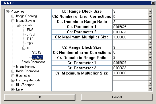
Finally, regarding custom settings, I can't explain much because that would expose proprietary information about my algorithm. Better to give the user the opportunity to experiment. After making settings in the simplified dialog, the user can click on a tree branch to switch to the custom dialogs. The user can then observe the resulting changes on the actual parameters and make additional changes on the actual parameters. If these custom savings are to be saved in sar.ini, the user should then click on the IFS branch and set Use Custom Settings to True. Greyscale images can be processed faster if Cb: Range Block Size and Cr: Range Block size are set to zero in the custom settings.
In the IFS algorithm, the input image is divided into adjacent, nonoverlapping blocks called "Range Blocks" and overlapping blocks called "Domain Blocks." For a W x H image, the number of range blocks is W*H/N2 , where N x N are the dimensions of the range block. The number of domain blocks is approximately (W-M)*(H-M), where M x M are the dimensions of the domain block. The user can select the range block size N and the ratio M/N = 2 or 3.
The algorithm matches every range block to a transformed domain block. The quality of the result depends on how well these matches are made. The reason that the quality of the result increases with the size of the input image is that the probability of finding good matches increases with the number of domain blocks. The IFS file records which domain block matches each range block and what transformations were made. When the IFS file opens, an output image consisting of range blocks is built out of domain blocks in an iterative process. You could say that the image is constructed out of pieces of itself starting with nothing but a set of rules contained in the IFS file. Image enlargement is accomplished by increasing the size of the range blocks in the output image, as this size is not part of the "rules."
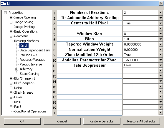
The default setting represent the Zhao modification of the Xin Li algorithm and NOT the original method. Only scale factors that are an integer power of two are directly permitted. However, if you enter zero, the dialog box for arbitrary scales will appear. Then Xin Li will be scaled to the next larger power of two and automatically reduced to selected size by using Lanczos interpolation. Parameters below the 3rd line of the 2X dialog are for use with miscellaneous and obsolete methods which can be ignored.

The scale factor is equal to two raised to the power given by the first parameter in the dialog box. This method is fast and does not produce jagged edges. It produces results similar to that of the original Xin Li method.
The following is optional. By using Resize>Set F2/F3 to Draw
Avoidance/Removal Regions, you can use the right/left mouse buttons to draw
Avoidance/Removal regions in red/green. You must select this from the
menu for each seam carving because a temporary copy of the original is saved
for seam carving. Removal will not work for enlargements. Don't
forget to change the mouse curser by pressing P.

The width and height must be between half and twice that of the original.
However, because the quality decreases substantially for increases more
than 50%, it is recommended that such size increases be done in stages with
derivative blending between stages.
Energy Function Mode Types:
0 - Sum of Absolute values of derivatives in Y channel of YCbCr color space.
1 - Sum of Absolute values of derivatives in all channels of RGB color space.
2 - Square root of sum of squared values of derivatives in Y channel of YCbCr
color space.
3 - Square root of sum of squared values of derivatives in all channels of RGB
color space.
4 - Sum of squared values of derivatives in Y channel of YCbCr color space.
5 - Sum of squared values of derivatives in all channels of RGB color space.
6 - Sum of Absolute values of derivatives in Y channel of YCbCr2 color space.
7 - Sum of Absolute values of derivatives in all channels of log RGB color
space.
8 - Square root of sum of squared values of derivatives in Y channel of YCbCr2
color space.
9 - Square root of sum of squared values of derivatives in all channels of log
RGB color space.
10 - Sum of squared values of derivatives in Y channel of YCbCr2 color space.
11 - Sum of squared values of derivatives in all channels of log RGB color
space.
Usually, the odd modes will produce better results but take more time than the even modes. More than other modes, modes 10 and 11 produces seams that tend to avoid passing through high contrast edges.
Update Energy Function - Apparently, in the original paper by Avidan and Shamir, the energy function was not updated between seam removals. Doing so (recommended) improves results at the cost of a small loss of speed.
Iterations for Derivative Blending ("Gradient Domain Seam Removal" or "Poisson Editing") - Zero is off. Usually, 100 iterations is enough. This reduces the severity of two kinds of artifacts:
1. Kinks in edges, ridges and lines.
2. Abrupt change of luminances in areas with previously slowly changing
luminances.
Also, textures often look better with derivative blending.
Blending Avoidance Weight - Setting this to a sufficiently large value prevents derivative blending from changing avoidance regions. Although rarely needed for size reductions, it is often needed for size increases.
Example input image:


Parameter Settings for following result:


Parameter Settings for following result:


Adding Avoidance (red) and Removal (green) Regions for following result:


Using the immediately preceding image as input with these avoidance regions,


Same as "Average" with radius = 1, but not conditional with mask and cannot be painted, i.e. you can select color channels only. Repeated application approximates a Gaussian blur with variance 2/3 N, where N is the number of iterations.
This can be masked and/or painted.
This operation simulates an unfocused camera lens. The user selects the Radius parameter to control the amount of blur. For variable lens blur, see Gradient Lens Blur. This operation can be painted and is conditional on both mask and color channel selection. Normally, only the result is masked; however, with the "Masked Input" parameter set to "True," masked areas will not be used as input. For example, suppose you have an image of stars in the night sky and you want to remove noise in the surrounding sky. To do this, mask the stars and use Average with "Masked Input" set to "True" to blur the noise. If this parameter was set to "False," the bright color of the stars would diffuse into the surrounding areas.
Multiple iterations of this filter no longer simulate lens blur. Instead, the result (with at least 3 iterations) will be a close approximation to a Gaussian blur.
This simulates blur caused by an object moving at constant velocity. The user selects the distance in pixels and angle in degrees.
The results from hysteresis, Farbman and bilateral filtering are very similar. All three remove/reduce texture/noise while preserving sharp edges. They can be used to produce the OPPOSITE effect, contrast enhancement, by linear extrapolation. For contrast enhancement, click Layers>Set F2/F3 to Add/Subtract, subtract smoothed image from original, then add difference to original by pressing F2 multiple times, Ctrl+F2 for fine adjustment. Alternatively, put blurred image in bottom layer, original in top layer, and use Layer>Set F2/F3 to Interpolate/Extrapolate Layers.
SAR 4.0 provides improved artifact reduction for hysteresis smoothing. The following example images show the types of artifacts and their reduction. The hysteresis smoothed results are shown on the left and the contrast enhanced counterpart on the right.
Original which you can use for testing: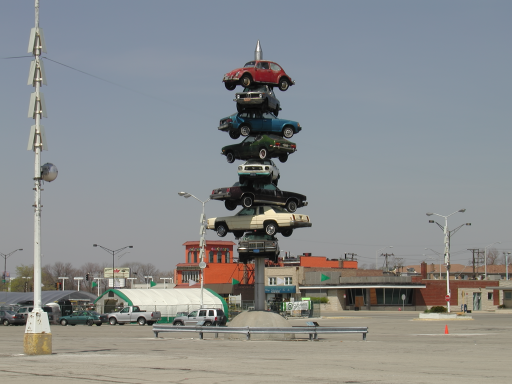
First, without artifact reduction:
Settings: (Tolerance=40, Iters=1, Combine Channels=False, Artifact Reduction=False, Iters for Halo Reduction=0):


Second, with artifact reduction:
Settings: (Tolerance=40, Iters=1, Combine Channels=False, Artifact Reduction=True, Iters for Halo Reduction=0):


Third, with both artifact and halo reduction:
Settings: (Tolerance=40, Iters=1, Combine Channels=False, Artifact Reduction=True, Iters for Halo Reduction=50):

Finally, when Combine Channels=True, there will be slightly more smoothing/contrast enhancement of color hue and saturation.
A repeat of the above with this setting follows:
Settings: (Tolerance=40, Iters=1, Combine Channels=True, Artifact Reduction=False, Iters for Halo Reduction=0):
Settings: (Tolerance=40, Iters=1, Combine Channels=True, Artifact Reduction=True, Iters for Halo Reduction=0):
Settings: (Tolerance=40, Iters=1, Combine Channels=True, Artifact Reduction=True, Iters for Halo Reduction=50):

Using more hysteresis iterations with a smaller tolerance, e.g., 8 iters. at 5 tol. instead of 1 iters. at 40 tol., will produce less halos and artifacts.


 ,
,
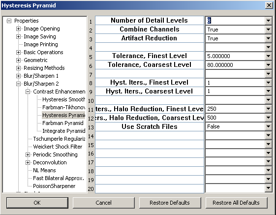
The Hysteresis Pyramid dialog box,
 ,
,
is similar, but the 5th and 6th parameter control the scale of detail images.
Again, you typically need not change other parameters.
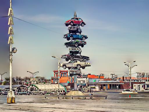
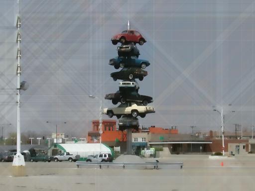
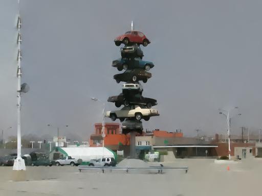
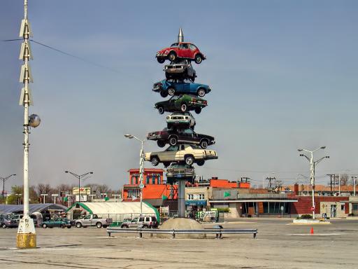
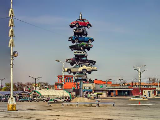
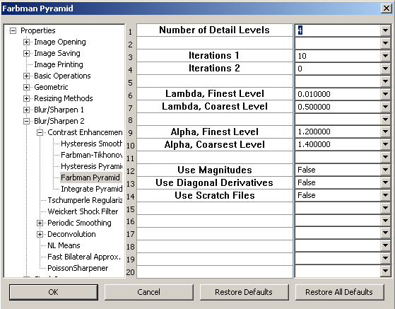
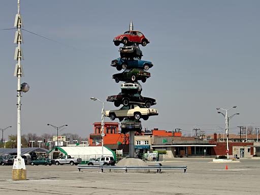
Using default Farbman settings, the car kabbob image was decomposed into the following base and four detail images:


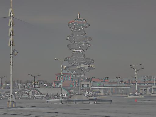


It should be strongly noted that the pyramid and results of integration depend on the initial color space. Typically, RGB and logRGB result in greater contrast of saturation and hue than HSV of HSI but take three times longer to process.
 ,
,
Integrate Pyramid automatically determines which channels apply from the color space of the input image forming the pyramid, i.e., user selection of channels have no effect.
For noise removal, I recommend that the "Window Size" (WS) be about the same size as the blotches of noise. Then use the minimum "Intensity Spread Factor" that removes the noise. Usually, this will be between 2.5 and 10. More than one iteration may be needed. If this produces posterization, the posterization can be reduced by additionally applying a few iterations with a small WS, e.g., 1, and larger IFS, e.g., 30.
This can also be used for various types of edge enhancement, such as removal of halos and sharpening. Also, edges are easier to detect after texture has been removed with the bilateral filter.
Similar to Average, but wmmr replaces average. Actually, there are several types of wmmr and this is the "median" type. Removes texture details while sharpening edges.
This causes curved edges to move toward the center of curvature. Small spots will become smaller faster than large spots. Useful for straightening jagged edges and lines, it is my experience that this is best applied to selected areas as a painted operation. It can also be used to remove impulsive noise, but, for this purpose, I see no advantage over median filtering.
The "Modulus" and "Offset" parameters are for experimental use in conjunction with removing jaggies from enlarged images. Under some circumstance, an enlarged image will contain some pixels that are unaltered from the original image. These pixels will be located at the intersection of every Mth row and column of pixels, starting with the Nth row and column. By setting Modulus = M, and Offset = N, these pixels are excluded from isophote smoothing, i.e., these pixels remain unchanged. Some people have claimed improved results, but I don't see it. If you are not experimenting with this, these parameters should be set to zero.
The "Modes" -1 and 1 refer to two different ways of implementing the algorithm. Since I noticed a very subtle difference in results, I included both. Mode 0 alternates between the two at each iteration.
Using "Average" mode and with "Sharpening Threshold" as the only threshold (other thresholds set to zero), this is equivalent to conventional unsharp mask. When the absolute value of the difference between pixel intensity values of a blurred and unaltered image is less than the threshold, the aforementioned difference is subtracted from original, thereby selectively sharpening areas of low sharpness.
The unconventional "Blur Threshold" and "NoOp Threshold" are thresholds below which the image is, respectively, blurred and unaltered. These can allow sharpening without enhancing noise. These thresholds are tested in order:
1. Blur
2. NoOp
3. Sharpening
All thresholds are expressed as a fraction of the color space range.
This produces less halos than USM.
Here are two examples using the car kabbob image.
(Sharpening Amount = 2, Scale Factor = 0, Poisson Iterations = 50).
(Sharpening Amount = 2, Scale Factor = 0.25, Poisson Iterations = 500).

The operation can now be masked and/or painted. It will sharpen, smooth, align edges, and remove halos. A disadvantage of Jensen is that it has a tendency to round corners. Curved edges tend to be moved toward the center of curvature.
New with v. 3.6, this can be used to remove purple fringing! You must use this in combination with YCbCr color space. Set to a window larger than twice the width of the fringing, set Use for Defringing to True, set Edge Detection Parameter 1 = 1 and set Edge Detection Parameter 2 = 0. It is recommended that defringing not be applied to an entire image. Either, manually paint to problem areas or unmask edge areas with edge detection before applying.
This is basically an edge sharpening filter.
This is for removal of semi-transparent repetitive patterns. The user may select one of two Pattern Type presets, crosshatch and honeycomb. When crosshatch or honeycomb are selected, the Number of Points and the Index Offsets are automatically calculated. Then the user need only enter Smoothing Function and Radius or Period of Repetition. Custom patterns can also be accommodated by manually entering Number of Points and Index Offsets, but further instruction on custom patterns will not be given.
Consider this example of an image with a honeycomb pattern:

The five steps to remove the pattern while retaining detail are:

In the example, I used the regular median filter (Blur/Sharpen>Median) with a radius of 4. Tip: For patterns that are faint and only visible in otherwise homogeneous areas, it might be better to use bilateral filter or Tschumperle regularization to obtain a "crude" start.


Observe that the pattern is of nonstationary intensity.

Observe that the process is less effective near the borders.
The image at this stage can be used as the final result or a faint remaining pattern can be further removed. You can remove a faint pattern using bilateral filter or Tschumperle regularization, spot retouch or globally, and repeat the process, substituting this for the intermediate result of step 1. The details in step 2. will be more faint and therefore more easily removed by a single repetition of periodic smoothing.
Finally, some adjustment of contrast and brightness is advisable.
You can make a disk (lens), uniform (rectangular) or Gaussian kernel with this. The latter two, if asymmetric, can be rotated by an angle given in degrees. Note that the kernel, as displayed by View Kernel below, is displayed with bottom to top order reversed and the rotation is as viewed. This can be a little confusing when rotating.
Find Kernel from Image of Point
If you have an image of a point source of light, such as a star, you can make a convolution kernel from it.
To use (ungrey) this menu item:
1. You must have only one color channel selected, e.g., Y of YCbCr color space.
2. The image of the point must be, at most, 35 pixel width and height (can crop).
Find Kernel from Blurred and Sharp Image
If you have a blurred and a sharp image of an otherwise identical scene, you can find or approximate the convolution kernel representing the blur.
To use (ungrey) this menu item:
1. You must have only one color channel selected, e.g., Y of YCbCr color space.
2. Two images of equal dimensions must be in the top and bottom layers.
With the blurred image in the top layer and the sharp image in the bottom layer, this operation will find a convolution kernel which, when convolved with the sharp image, approximates the blurred image. Sometimes, especially with slight blurs, by reversing the top and bottom order of the images, you can get a kernel that, when convolved with the blurred image, effectively deconvolves (sharpens) it.
Once a kernel is made or found, you can save it in binary form by selecting a file name with a ".kernel" extension or a text file with a ".txt" extension.
You can also write a kernel text file with notepad, for example:
5, 3,
1/15, 1/15, 1/15, 1/15, 1/15,
1/15, 1/15, 1/15, 1/15, 1/15,
1/15, 1/15, 1/15, 1/15, 1/15,
Every number must be followed by a comma.
The first two numbers respectively represent width and height which must be odd integers.
The numbers that follow are the kernel entries which can be fractions, decimal or scientific notation.
They are in order of increasing memory address.
Opens a file previously saved per above thereby creating a kernel.. Be forewarned that there is not much error checking on this.
This operation produces temporary text files representing the kernel and opens them with Window's Notepad. The format specifier is in C language. For example, in "%16.8", "8" is the number of digits after the decimal point and 16 is the spacing between numbers.
You also have the option of viewing the Singular Value Decomposition (SVD) of the kernel, however, the number of columns cannot be less than the number of rows.
The reason for viewing SDV is that often convolution can be performed much faster when done as a sum of a few separable convolutions.
In the Convolution and Deconvolution to follow, you have the option of doing this to increase the speed of calculations.
For example, this is a lens kernel:

Direct convolution with this kernel takes 7*7 = 49 multiplications per pixel.
Now inspect the center (following "7,1,") row of the SVD:

These values are always positive and listed in descending order.
Since only the first two values are relatively large, we can approximate convolution with this lens kernel with four one dimensional convolutions involving the first two rows of the top and bottom matrices.
Such convolution takes 2*2*7 = 28 multiplications per pixel.
Note that because only the first four values nonzero, using the first four row pairs would result in exact convolution but that would take 4*2*7 = 56 operations per pixel.
The following is a visual depiction of the SVD kernel approximations using 4 (upper left), 3 (upper right), 2 (lower left) and 1 (lower right) row pairs.

When you are done using the kernel, you should destroy it to avoid memory fragmentation.

Referring line 1 in the above dialog box, setting Use SVD to False will perform direct convolution of the image with the kernel. Setting to True, indirect convolution will be performed using the number of row pairs specified on line 2. Setting line 3, Normalize to One, to True insures that flat regions will not change in brightness. If line 4, Report PSNR, is set to true AND there are two layers, the Peak Signal to Noise Ratio of the difference between layers will be reported in the 5th pane of the status bar.
The only parameters that you need to change below line 9 are those on lines 10 and 11. Typically, these values should be decreased for noiseless images when the convolution kernel is accurate. Typically, the 1:2 ratio between the two parameters should not be changed much. The other parameters are for experimentation until I can advise better. Maybe, on line 14, PseudoTotalVariation is a safer choice than the default, Huber Estimator 2 Pass; in any case, it will be faster. See exercise4

After creating or loading a profile, use this operation to process different images with similar noise. This has a default profile, but, if you use the default profile, results will probably be bad.
First, you should create a noise profile by selecting a rectangular area in a relatively flat region of the image such as blue sky. This operation will remain greyed out until you select a rectangular region. Do that by dragging the mouse cursor while holding the right mouse button and Control key down. Important! You must select a color space, typically YCbCr (CSpace>YCbCr), which becomes part of the profile but it is not displayed in the dialog boxes. If you use the above default parameters with the default RGB color space, the results will be awful! The color space is displayed in the second pane of the status bar. After clicking Create Noise Profile, the following Dialog box will appear.
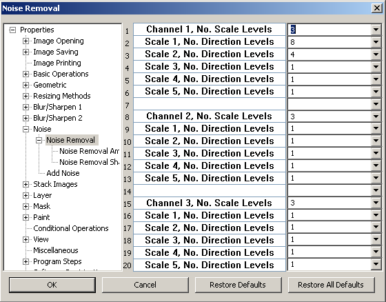
The parameters in this dialog are used in relatively slow preliminary calculations that are repeated with every new image. The results of these calculations are stored in temporary files that are automatically deleted when SAR closes. These default parameters in this dialog box are for YCbCr, YCbCr2, YUV or "YCbCr Gamma X" and I suggest that you leave them alone unless something goes wrong. Incidentally, if you selected YCbCr, YCbCr2, or YUV and more noise remains in darker than lighter regions, as is often the case, use "YCbCr Gamma X." On lines 1, 8, and 15 you select the number of levels between 1 and 5. You should select more levels only if the noise has has a relatively coarse appearance. The other lines select the number of contourlet directions except "1" which selects wavelets which are much faster to calculate than contourlets. The reason that you see asymmetry here is that the Y channel is more important than the Cb and Cr channels, so the slower contourlet calculations are only performed on the Y channel. However, if for some odd reason, you wanted to use RGB color space, then the parameters should be made the same in all channels. After closing the above dialog, two more will appear:

The above controls the amount of noise removal. On line 2, you have the option of getting the PSNR reported in 5th pane of the status bar. To use this, you must put a noise free image in the bottom layer and a noisy version in the top layer. The noisy version could be produced by adding artificial noise to a noise free version. Or, alternatively, the noise free version could be produced by stacking multiple frames of the same scene and the noisy version could be a single frame.
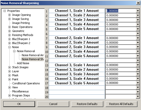
The above controls sharpening.
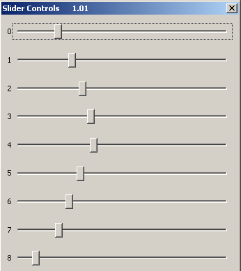
The parameters of the last two dialog boxes involve relatively fast calculations. You can enter these parameters by using sliders which appear after closing these dialog boxes. Again, I emphasize that you can afford be sloppy with channels other than the Y channel which must be carefully tuned. After doing it once, you can quickly redo the slider adjustments with "Redo Same Image." For some reason I don't know, typically, only sharpening the second level (line 2 in the last dialog) increases PSNR.
This is greyed out until you use Create Profile or Noise Reduction by Contourlets. Use this to quickly repeat adjustment of parameters in the above last two dialog boxes.
PCA based noise reduction is the best practical noise reduction method in SAR image processor. Although slow, it is not impractically slow and my tests show that, with fine tuning, it usually produces better results than Topaz Denoise. If you want faster processing with inferior results, use Noise Reduction by Contourlets.
First, form a rectangle of at least 50x50 dimensions in a homogeneous region of a representative image as shown here:

The above rectangle is formed by dragging the cursor with the right mouse button down and holding the CONTROL key down while releasing the right mouse button.
If you do not hold the CONTROL key down, the image will be cropped and this procedure will not work.
Then, select menu item, Create PCA Matrices, which will become ungreyed.
This dialog box will appear:

Usually, the default settings of parameters above line 15 will be adequate. Here, it is better to use the whole image rather than a crop, even though I didn't on the present example. Setting Denoise Now, line 16, to "False" will cause the current image to be unprocessed but small matrices are stored in RAM for later use. When you are done denoising you should free RAM by removing these matrices with menu item, Destroy PCA Matrices. Color Space Automatic Conversion, line 18, is important. If there is too much smoothing in the dark or light regions of an image, select YCbCr Gamma X and adjust the parameter on line 19 by trial and error Increasing/decreasing gamma above/below 1 will increase/decrease smoothing in dark/light regions.
Setting Denoise Now, line 16, to "True" or later selecting menu item, PCA Based Noise Reduction, will cause two more dialog boxes to appear:

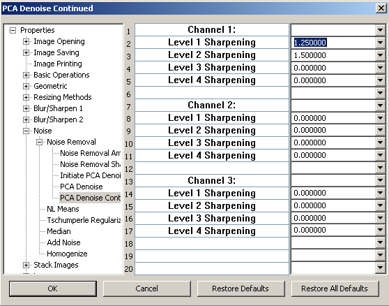
The reason that the default noise reduction amount is less for channel 1 than for channels 2 & 3 is that more noise reduction in the Cb and Cr channels makes the results look better. With PCA Based Noise Reduction (menu item), it makes no difference whether the image is cropped or not, therefore you can use a small crop to save time while adjusting the parameters in the second dialog box (but not the first dialog box) by trial and error.
Here is the result using default parameters:

Because this is very slow, it is only practical for use on very small images. Also, there is considerable tradeoff between quality and speed with respect to the parameter settings. For maximum quality, the Search Radius should be set to half the maximum image dimension. Doing this, will cause the operation to practically take forever.
This algorithm was developed by Dr. David Tschumperl� for his Ph.D. Thesis. The version presented in SAR's Blur/Sharpen menu is particularly useful for removing certain types of noise. Another version is presented in SAR's Paint menu for inpainting. I have made several modifications.
The amount of effect is controlled by both the number of iterations and the step size. There are two step size parameters, one for blur and one for edge contiguity. In the original algorithm, these were equal except, for inpainting, blur step size was zero. Larger step sizes allow fewer iterations, however, unwanted artifacts are likely to appear in homogeneous regions. I have also provided a "Blur Parameter" and "Edge Parameter" to help control these artifacts. Higher values tend to reduce the aforementioned artifacts. In the original algorithm, these were both set equal to one.
The "Mode" parameter selects one of two ways that discrete derivatives are calculated. Mode 1 is the original used by Dr. Tschumperl�, whereas Mode 2 tends to produce sharper diagonal edges.
In the original algorithm, certain quantities were recalculated at every iteration. I found that recalculating these quantities only on every 10th or 100th iteration results in a substantial savings in time with little loss of quality. The user controls this with the "Recalculation Interval" parameter. If the Recalculation Interval is set to one, recalculation is performed as in the original algorithm.
This is intended for use with RGB color space, but the user has the option to experiment with other color spaces. This operation cannot be separately applied to individual color channels, but it can be masked and/or painted.
1. Generate an unmask on all black regions using Mask>Set F2, F3 to Mask by Color.
Notice that the edges of the black lines became ragged.
This unwanted effect can be reduced by working with larger scans or enlargements and then reducing the size of the results.
It's better to work with larger images anyway because it is easier to see the line gaps that need to be painted closed.
Combines multiple pictures of identical or slightly changing scenes from files
selected with a file opening dialog box. In this dialog box, you
make multiple file selections the same way you would with Windows
Explorer. During processing, the number of images is counted in the
fifth pane of the status bar.
Attention! Images must be in alignment. If not in alignment, the
images must be digitally aligned before stacking. See,
How to Align Images from Hand Held Camera
, below.
SAR has six modes:
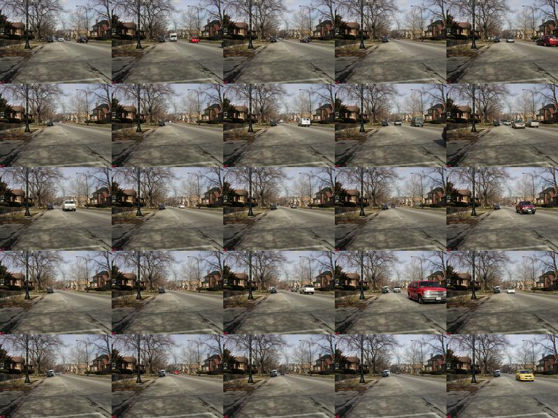
The following shows 25 exposures of a street with passing cars.
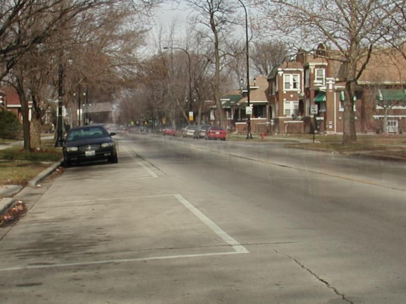
The following is the cropped result of regular Average stacking on those
images. Observe that ghost-like images of the passing cars,
especially along the center of the street.
The following is the cropped result of Multivariate Median 2 stacking on those
images. Observe that almost all traces of the passing cars were
removed.
http://www.janrik.net/ptools/ExtendedFocusPano12/index.html
http://helicon.com.ua/pages/focus_samples.html
Some of these images first need to be aligned (see below). I think you
will find that SAR's Extended DOF outperforms the competition with respect to
both quality and speed.
Homogenize Insides of Line Enclosures
This homogenizes the color of regions enlosed by an unmask.
It is most useful for undithering scanned cartoons like this one:

2. Remove small spots on the mask with Mask>Remove Small Spots.
3. With Mask>Set F2, F3 to Clear/Set Mask, remove gaps in unmasked lines to prevent otherwise separately colored regions from being treated as one region.
4. Invert the mask. The regions to be homogenized will be temporarily displayed in black. (This display of black can be removed with S key.)
5. Use Homogenize Insides of Line Enclosures. This is the result:

Stacking (Regular and Modified)
Warning! All modes, except Average and Extended DOF,
create temporary files (in the same directory as sar.exe) which use a huge
amount of hard disk space. Failure to supply adequate disk space
(several GB recommended) will result in a crash. If this happens,
these temporary files will remain. To remove these files, simply
open and close sar.exe .
Multivariate Median Example:

Extended DOF Examples:
My digicam doesn't have sufficient focus control to produce suitable images,
but here is a link to test images from competitors:
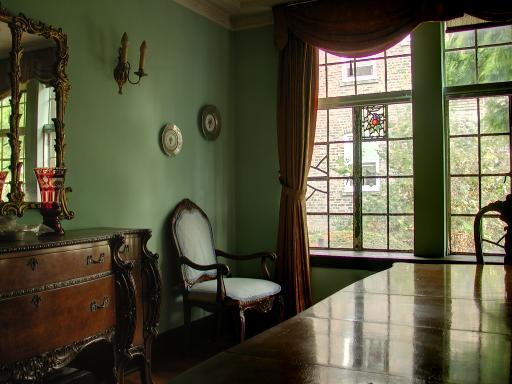
Extended Dynamic Range Stacking Example:
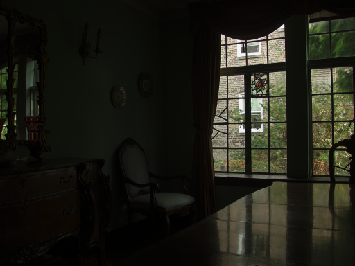
Using a tripod, five sets of five pictures, each set representing a different
exposure time, were taken of the same scene. The five images in each set
were stacked (averaged) to produce these results.

Then the five images were stacked using Extended Dynamic Range Stacking to
produce this result (48 bit PNG):
You can use this as a test image for tone mapping. It will be processed
by tone mapping below.
This makes a greyscale template from the image to which other images will be aligned. The alignment operations are disabled until this template is created.
Because the alignment template uses large amounts of RAM, it should be destroyed after use.
Typically, you will use a tripod and interval timer to take pictures for stacking. Even so, wind or manual camera adjustments may cause small shifts between images. This operation is mainly for aligning such images prior to stacking. To enable this, you must first create a template from an image, after which, pressing F2 will quickly align a similar image to the one used in creating the template. Alignment may fail if the image is misaligned by more than 1/3 the minimum dimension of the image. During alignment, portions of an image extending beyond its border will be wrapped around to the opposite side. After finishing all alignments, you should destroy the template to free RAM. If used in Batch processing, there is a setting in the Batch dialog box that automatically destroys the template at the end of Batch processing. It typically takes 1 second to align a 3.3 MP image.
Attention! This operation is usually necessary for accurate alignment of images from a hand held camera! There are two versions of this operation, one found under Stacking, another found under Layers. Both share the same parameter settings. The difference between the two is that Stacking version aligns images to a greyscale "alignment template" whereas the Layers version aligns the top layer to bottom layer using all color channels. The Stacking version is about three times faster but slightly less accurate. This operation first finds shifts in small non-overlapping blocks and then interpolates these shifts to align images. Although only shifts are involved, this alignment procedure can compensate for many different kinds of distortions, including small rotations. It is important to set the Search Radius greater than the maximum misalignment in pixels. However, the greater the search radius, the slower the operation. Typically, images previously aligned by Set F2 for Rotational/Resized/Translational Alignment (below) will be within 3 pixels, the default search radius for Elastic Alignment. For Elastic Alignment, it is important that the alignment template not contain passing objects. For Rotational/Resized/Translational Alignment, passing objects are much less deleterious. The nominal accuracy of SAR's Block Alignment is 0.0625 pixels.
This is for aligning images taken with a hand held camera. Although not unreasonably slow (about 1 minute for a 3.3 mp image), this operation is not perfectly reliable therefore images should be inspected after using this operation for accurate alignment. Similar to Geom>Arbitrary Rotation, unknown portions of the image will be filled with reflections.
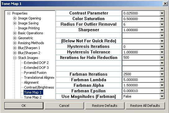
This is loosely based on the method presented in this paper:
K.K.Biswas and S.Pattanaik, "A Simple Tone Mapping Operator for High Dynamic Range Images," School or Computer Science, University of Central Florida This can be used on normal low dynamic range images by setting the Contrast Parameter equal to zero.
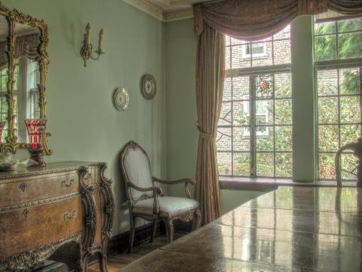
This is the result of processing the previous Extended Dynamic Range image:

using default settings:
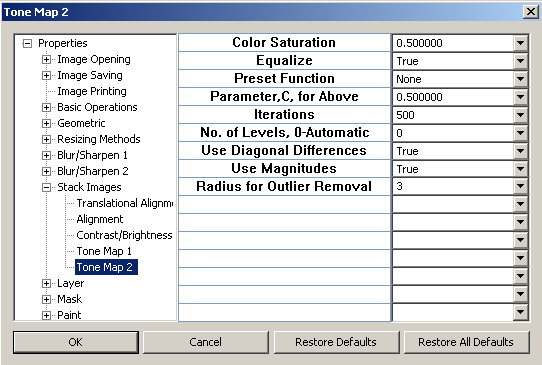
This is based on the method presented in the papers at http://www.mpi-inf.mpg.de/~mantiuk/contrast_domain/
This is the result of processing the previously stacked image:
using default settings. Typically, a Tone Map 2 result will benefit from
post sharpening.
The following was sharpened using the Poisson Sharpener:

Tone Map 2 involves an iterative process that can take up to 1500 iterations to become visually stable. The iterative process is initiated with a black (0,0,0) image. During early iterations, sharp, local features appear first. Thus, a small number of iterations, e.g., 50, will result in a sharper image with possible halos. As iterations become increasingly large, e.g., 500, the image will be less sharp but have negligible halos.
The Radius for Outlier Removal is explained under Basic >Scale and Shift to [0,255].
There are advantages, other than convenience, to stacking digitally aligned images from a hand held camera instead of from a camera with tripod. After digital alignment of slightly misaligned images from a hand held camera, JPEG artifacts, demosaicing and other sensor based anomalies will occupy random positions and therefore be reduced as noise by stacking.
You should align an image set in at least two stages, first, by using one image from the set as a template, and, second, by using the result of multivariate median stacking of the first aligned set as a template. It is done this way because noise and passing objects in the first alignment template will contribute to inaccuracies in the first set of aligned images. Multivariate median stacking will reduce noise and passing objects from the template used in the second stage.
I can't anticipate all contingencies, so, please, use common sense; I want this to work for you.
1. Try to select a good image from the set to be aligned. You can optionally make rotational adjustments on this. Create an alignment template from this image.
2. If the exposure of every image in the set is visually similar, skip step 2 and go to step 3. Otherwise, e.g., there was variable shade from passing clouds, create a Brightness/Contrast template and use Set F2 for Brightness/Contrast and batch process so the images have similar brightness and contrast. This is necessary because the multivariate median stacking used in step 4. does not perform well with variable exposures.
3. Batch process the images with Rotational/Resized/Translational Alignment.
4. Stack the aligned images using Multivariate Median.
5. Create a new alignment template using the multivariate median stack result. This is done to remove passing objects from an alignment template so that the passing objects won't interfere with Elastic Alignment.
6. Starting with either the original set or the brightness/contrast adjusted set, use Rotational/Resized/Translational Alignment followed by Elastic Alignment . You can either do this as two batch processings, or you can combine the two operations into one action and apply in one batch processing.
7. Although rarely necessary, for extra accuracy, you can repeat starting with step 4.
8. Tips: Use copies of your original files so you don't lose them by accident. A good file format to use for batch processing output is 16 bit/channel PNG. After batch processings, it is often useful to inspect intermediate results with Sequential Load (F9).

If the top and bottom layers are of different dimensions, this will match the sizes of the layers. The images contained in those layers will be retained and positioned with coincident lower left corners.
Pixel values at corresponding coordinates throughout the images are added/subtracted.
Tip: This can be used to incrementally sharpen images. Exchange layers and duplicate image in bottom layer (=). Then blur the image and subtract the bottom layer. Exchange layers again and use F3 to sharpen image.
The F2 "Interpolate" operation is represented by the following equation:
(1-C)*(top image) + C*(bottom image)
where C is the parameter entered in the dialog box. In other words, the result is a weighted average of the two images. The F3 "Extrapolate" operation is the inverse to this weighted average.
Tip: This, also, can be used to incrementally sharpen images. Exchange layers and duplicate the bottom layer (=). Then blur the image and exchange layers again. Set F3 to Extrapolate and use F3 to sharpen image.
Similar to Lens Blur except variable radii values are given by pixel intensity values in bottom layer. See Gradient and Lens Blur.
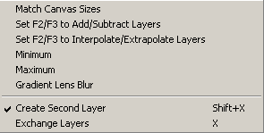
This toggles creation and destruction of a second layer. No more than two layers can be created. These layers consume a lot of RAM.
Creates a second layer with the same dimensions as the first. (The new layer will contain a black image.) However, the two layers will not necessarily remain the same size because, afterward, the size of each individual layer can be independently changed. Bear that in mind, because most operations that simultaneously involve both layers are disabled when the dimensions do not match. The old layer and newly created layer are respectively designated as "Layer 1" and "Layer 2." Either layer will be called the "top layer" when it is normally visible and either layer will be called the "bottom layer" when it is normally invisible. Operations involving only one layer are applied to the top layer. The top layer is indicated in the fourth pane of the status bar. Also, the existence of a second layer is indicated on the menu bar as "Layer( On)."
When a second layer is destroyed, it is always Layer 2 (even if Layer 2 is on top).
Exchanges the top and bottom layers. If there is only layer, a second layer will be created.

A typical procedure for cloning involves moving the bottom layer around (e.g., Shift+Arrow, Alt+Shift+Arrow) while viewing it through an unmasked region (toggle Shift+S for peer through). When a suitable underlying region is found, pressing F2 will transfer the it to the top layer. Don't forget to turn off the peer through by toggling Shift+S, or you won't see the result.
This is a sophisticated modification of the above which blends the boundary and, to a lesser extent, the interior of a region transferred from the bottom to the top layer. It is most useful for cloning textures, e.g., skin textures, removing tattoos, etc. This operation is always applied to all color channels and there must be a mask with an unmasked region OR the operation must be painted. Of course, painting can be used in combination with a mask. The derivative blending is an iterative process and the result depends on both the number of iterations and the starting point.
Example:
Original:

Cloned without derivative blending::

Cloned with derivative blending::
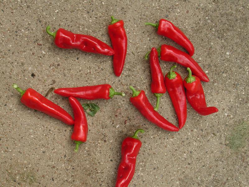
This is used to tile images like this:
First, you must create a blank canvas and put it on the bottom layer. You can do this Geom>Create Blank Image, followed by pressing the X key. Then, load a smaller image to be tiled. Next, select Set F2 for Tiling Top into Bottom from the menu. This initializes the operation so that, the first time F2 is pressed, column and row counters are initialized. Also, the first time you press F2, the top image will be transferred to the upper left corner of the bottom layer, after which the bottom layer will be copied to the top. Repeatedly loading new images and pressing F2 will continue the tiling from left to right and top to bottom. If you need to start a new tiling, don't forget to reinitialize again by clicking Layer>Set F2 for Tiling Top into Bottom in the menu. This operation can be combined with image size reduction using Prog>Record Program and/or used with File>Batch Operation, but don't forget to reinitialize.

These are used to match the colors of one image to those of another image of an identical or similar scene. The resulting polynomial coefficients can be applied to other images. The results depend on color space. Sometimes a PCA conversion (under CSpace) is useful (I don't know why). First degree polynomials compensate for histogram shifts and expansion or contraction. Higher order polynomials are for nonlinear transformations such as gamma.

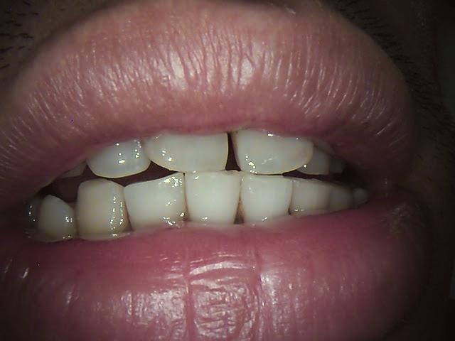
Referring to the above dialog box, to match aligned images of identical scenes, set Use Sorted Values, line 12, to False. To match images of similar, non-identical scenes, set Use Sorted Values, line 12, to True. Here are two images of two similar (approximately equal areas of teeth, lips and skin), but not identical scenes:
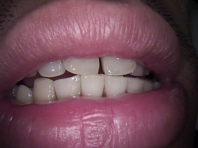
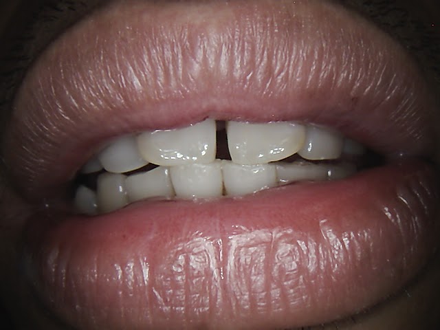
This is the resulting color match of the first image to the second using a 4th degree polynomial and a PCA conversion of RGB color space:
This works best in log RGB or log CMY color spaces. Top and bottom layer images must be of the same scene and aligned. Roughly speaking, this operation matches portions of the histogram of the top layer to portions in the bottom layer.

These boolean operations between masks in top and bottom images are stored in the top mask. These operations can be painted.

Displays a weighted average of top and bottom layers (RGB only). This is useful for manually aligning dissimilar images via One Point Registration and Ctrl (or Shift) + Arrows keys.
Displays absolute difference of top and bottom layers (RGB only). This is useful for manually aligning similar images via Ctrl (or Shift) + Arrows keys.

This feature is enabled when equal sized images are in the top and bottom layers. It reports statistics on the differences between the two images. This feature can be used to compare the quality of results from different enlargement methods. First, a large original is reduced, usually using box interpolation. Then this reduction is enlarged to original size by the method being tested. The statistics on the differences between the enlargement and original serve as objective criteria for determining which enlargement method is best. The most commonly used measurement is Peak Signal to Noise Ratio (PSNR) (larger is better). Alternatively, one can use Root Mean Squared Error (RMSE) or Average Absolute Error (AAE) (smaller is better). AAE is less sensitive than RMSE to a a few large errors. However, these measurements do not tell the whole story. All else equal here, structured errors are worse than unstructured errors, but, to my knowledge, nobody has quantified this yet.
New with version 4.2, Mean Structural Similarity Index (MSSIM) is optionally included. Select it on line 5 below.
Here is its FFT (actually the magnitude):

Notice that the dimensions of the FFT are the nearest greater integer power of two, in this case, 1024x1024. An FFT is in two parts, the other part, phase, is in the bottom layer and will not be used except to take the inverse FFT. I paint an unmask on the high frequency peaks in one quadrant, reflect across middle horizontal and vertical lines and set the unmasked regions to zero with Shift+Z to get this:

Then, I take the inverse FFT to get this:
Notice the dithering is gone.

All masks are binary. Most of the following mask operations will create a mask when one doesn't already exist. By default, unmasked regions will be displayed in black. This "black" is not saved to file or printed, it merely shows you which part of the image is unmasked and masked: the black areas are unmasked and non-black areas are masked when Mask->Show Unmasked Area is checked and visa-versa when Mask->Show Masked Area is checked. Press S key to toggle this display feature. Also, there are other mask display options. In particular, you can see a bottom layer through an unmasked region of the mask on the top layer by using Shift+S.
When a new image file is opened (except for FDIB files), if the new image has the same dimensions as the image that it replaces, the mask of the old image will be retained. If the new image has different dimensions than the old, the old mask is destroyed. FDIB files store the mask with the image.
Toggles mask creation and destruction.
Creates a one bit depth mask for the top layer. Upon creation, all mask bits are zero (all pixels masked). The mask can only be saved with *.fdib image files. The existence of a mask is indicated on the menu bar as "Mask( On)."
Sets F2/F3 keys to set mask bits to 1/0. This operation can be painted.
This operation is conditional upon color channel selection. Also, some color spaces will show advantages over others.
This operation unmasks edge areas of the image. Unmasked areas will be displayed in black. F2/F3 increments/decrements a tolerance parameter such that F2 increases the unmasked areas and F3 decreases the masked areas. When recording actions, individual key pressings are not recorded, only the final tolerance.
Masked areas become unmasked and vice versa.
Extends the edge of an unmasked area by one pixel.
Useful for Noise>Homogenize Insides of Line enclosures.
Draws horizontal and/or vertical bars. This involves a departure from SAR's convention of having a coordinate origin at the lower left corner of an image. Here, the origin is the upper left corner because 8x8 JPEG blocks start there and this mask feature is useful for blurring the border between JPEG blocks.

Displays unmasked areas in black.
Displays masked areas in black.
When checked, the cursor should change shape and become a circle with a dot in the center. The diameter of the circle is controllable with the numerical keypad + and - keys. There is a bug under Windows ME/98 such that the cursor does not change. The size and appearance of the cursor can also be controlled from the Properties Dialog which will appear when the Ctrl key is held down while clicking Paint.
By holding down the right mouse button and dragging the cursor, most F2 programmed operations can be painted. The swept area will temporarily appear black and the operation is applied upon releasing the button. Similarly, the middle mouse button paints F3 programmed operations. With "Cond(Off)" painting is unaffected by a mask. With "Cond( On)" painting is applied only to the intersection of unmasked regions with the area swept by the paint cursor. If operations that can be painted are combined in an action, the action can be painted.
Set F2 to Smudge
See Exercise 5
See Exercise 6
The time for this operation increases with the number of unconnected paint strokes and small unconnected strokes count almost the same as large unconnected strokes. Therefore, it is advisable to connect strokes of a single color when possible. By "color," I mean the combination of hue and saturation represented by the Cb and Cr channels of YCbCr color space.
Mode 0 is default and mode 1 is experimental.
Mode 2 is for recoloring a color image. Change the color image to greyscale, put it in the top layer and put the color version in the bottom layer. Information from the colored version will help the recoloring process. Otherwise, everything is done the same as in Exercise 6.
I rarely use this anymore because seamless cloning is better in almost all situations.
1. Select an appropriate color space, usually YCbCr.
2. Select a rectangular textured area as shown, for example, in this figure:
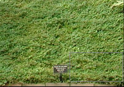
This is done by holding the right mouse button down and dragging the arrow cursor as in crop, but hold Control key down when releasing mouse button to prevent crop.
3. Then click on Record Texture which should now be enabled.
4. Click Set F2 for Texture Inpainting.
5. The texture can now be masked and or painted. The sign in the figure below was painted over.

6. When you are done with this operation, click Destroy Texture (formerly Record Texture) to release memory used for texture recording.
The textures are drawn in a diagonal direction from top right toward bottom left and, as such, tend to be congruent with areas adjacent to mask edges facing the top right and incongruent with other areas. Also, lines within a texture and approximately parallel to the drawing direction are well preserved. The drawn textures are based on pseudorandom numbers and are, therefore, different every time drawn. Thus, it is recommended that areas be painted several times until a result that is pleasing to the eye is achieved.
I have found this useful for accurately simulating digicam noise or film grain in otherwise noiseless digital images. The procedure follows.
A. Use logCMY color space.
B. Find a small, e.g., 100x100, homogeneous area with noise or grain to be simulated and crop it. (By "homogeneous," I mean homogeneous except for the noise or grain.)
C. Duplicate this to a second layer.
D. Blur out the noise in one layer, e.g., with 1000 iterations of Fast 3x3 Average, and then subtract this from the unblurred layer. (With logCMY color space, the result will appear mostly white but with noise or grain.)
E. Use this result to Record Texture.
F. Destroy the second layer and load the image to which you want to add noise. (You should still be logCMY space.)
G. Create a second layer by pressing X. (This will appear white.)H. Set F2 for texture inpainting and press F2. You now have a simulated transparency, almost clear except for noise or grain.
F. Add the two layers. The result will be like a print made from two
stacked negatives, one without noise or grain and the other clear except for
noise or grain.
This fills unmasked areas so that outside edges connect. In the example below, the black, unmasked areas are inpainted.

This is done in two stages which can be performed separately or together. The first stage is turned off by setting Initialize to False and the second stage is turned off by setting Iterations to zero. The first stage serves as a quick initial approximation and is simply a blurring of masked pixels into the unmasked regions. In the example, the result of the first stage is shown in middle. The second stage is the actual Tschumperle inpainting. The result of Tschumperle inpainting is shown at the bottom of the example image. The wider the gap to be filled, the more iterations are necessary. With the first stage turned off, the Tschumperle inpainting can be applied in cumulative steps by pressing the F2 key repeatedly until the widest gap is filled.
The Dominant Channel parameter provides some modifications to the original algorithm. In the original algorithm, certain calculations were based on all color channels. With the default parameter value, "Combined," there is no modification. However, this somewhat restricts proper operation to RGB color space. The other values allow proper operation in other color spaces. In particular, "Automatic" or "X" works well with the YCbCr color space.
For an explanation of the other parameters, see Tschumperle Regularization under Blur/Sharpen.
Tschumperle inpainting can be used to remove jaggies from some enlargements.
Under certain circumstances, an enlarged image retains all of the pixels from the original image. These unchanged pixels are periodically dispersed in the enlargement and need to be masked before applying Tschumperle inpainting. If the following conditions are met, this operation will mask the proper pixels.
1. Enlargements are made by SAR's bilinear, bicubic, Lanczos, triangulation or Xin Li interpolation.
2. The scale of the enlargement is an integer.
3. For odd integer scales, the image is centered. (This excludes Xin Li.)
4. For even integer scales, the image is off center by one half pixel in both horizontal and vertical directions. This is the default state for Xin Li; however, for the other interpolation methods, the user should set Horizontal Offset = 0.5 and Vertical Offset = 0.5 .
5. The scale parameter is properly set in the dialog box.
If the image was enlarged under other circumstances, there may be no unchanged pixels in the enlargement or they may have other locations. In either case, the mask generated by this operation will be useless.
You can check whether a pixel is from the original to make sure that it is masked. If the original was from an 8 bit per channel file, the RGB values of unchanged pixels in the enlargement will be integers, whereas the RGB values of interpolated pixels will almost certainly not be integers. You can examine the RGB values of any pixel by left clicking the mouse cursor on it. The RGB floating point values will appear in the rightmost brackets of fifth pane in the status bar.
Unlike inpainting unknown areas, with enlargements, it is usually undesirable to iterate to equilibrium because it is often desirable to retain some of the character of the original enlargement. Thus, it is recommended that one use the minimum number of iterations necessary to remove jaggies.
Finally, a warning. Before using Tschumperle on an enlargement, make sure that the Initialize parameter is set to False. Otherwise, the initialization stage may take days to complete and produce a bad result. Of course, in that case, it is better to give SAR the three finger salute (Ctl+Alt+Del).
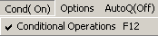
When checked, most operations (when possible) will be conditional on the color channel selection and/or masking. This is always on at startup. "Cond( On)" as opposed to "Cond(Off)" appears in the menu bar. Use F12 key to toggle on and off.
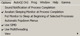
When checked, a WAV file is played when an operation is completed. The user must supply the WAV file, rename it sar.wav, and place it in the same directory as sar.exe. I use Sam Kinison's Yell
With this option set, a menu will appear as soon as the mouse cursor hovers over a menu bar item. (I also wanted the menu to disappear as soon as the cursor is placed off the menu, but that is beyond my Windows programming skills.) If you accidentally open a submenu, you can close it with F10 or click on main window.
This is now the default option selected by Options>Use Multithreading. Multithreading does not apply to all operations selected directly from the menu, but it applies to all applied with F2 and F3. Also, it applies to almost all operations that display a progress bar (from menu or not).
Previously, not having multithreading caused many problems while an image was being processed, including
Now, with multithreading, most of these problems are gone. A notable exception is that, during resizing, the image display may go blank because the original image no longer exists in RAM. During resizing, the RAM occupied by the original image is scavenged because all available RAM may be needed. Otherwise, during image processing, you can now manipulate the image display with the arrow keys, F5, F6 and resize the window. By setting Q>Miscellaneous>Thread Priority to IDLE, there will be negligible interference with other programs.
With previous versions of SAR, users were advised to run SAR in Windows 98 compatibility mode; don't do it anymore. This newly implemented multithreading is likely to be fraught with bugs. If something goes wrong, uncheck this option.

Set so that image display is resized to fit the client area of the screen. This only affects the display and not the image. The interpolation method can be selected in the Properties Dialog, which can be invoked by holding down the Ctrl key while clicking menu item. Microsoft's "Halftone" method is fastest; however, I have noticed that results differ between Windows XP and ME. "Show Combined," "Show Difference" and F7 (below) are not compatible with Halftone, but are compatible with the other methods. None are compatible with "Show Masked Area," "Show Unmasked Area," and "Show Bottom Layer Through Mask."

The first pane shows the image dimensions. The second pane shows the color space. The third pane shows the active color channels. The fourth pane shows which layer is on top. The fifth pane shows left click pixel information. Also, the fifth plane displays information for Batch Operation, Sequential Load, and Iterated Function systems. The sixth pane gives the time that it took to complete the last operation and a progress bar for resize and other time consuming operations.
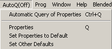
When this menu item is checked, the properties dialog will automatically appear before an operation to allow adjustment of parameter values. The default is checked.
A single dialog box gives the user access to almost all parameters. These parameters are saved in the sar.ini file when SAR closes and loaded the next time SAR opens. Clicking on a tree item on the left side of the dialog box will bring up an associated list of parameters and "combo" edit boxes on the right. Upon opening, the current value of the parameter will be displayed in an edit box. When the user enters a selection into the edit box, that selection does not take effect until the user activates the OK button or when another tree selection is made. If an entry is improper, e.g., outside allowable limits, the old parameter value will be retained. Often, values are not limited to those that appear in the drop down list under the edit box. To inspect whether your entry was accepted, without closing the dialog box, click on another tree item and then click back.
Sets dialog box properties, with the exception of registration key code, to default values.
Sets color space to RGB with all channels checked, 2nd Layer off, mask off, paint off, and Conditional on. This action is recordable and should be used to initialize some programmed actions in order to prevent the program from toggling the aforementioned items to the wrong states.
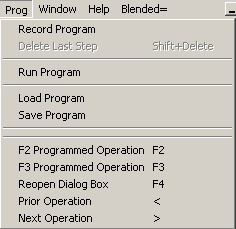
These menu items represent the F2 and F3 keys. The name of the operation programmed into the F2/F3 keys replaces "NoOp" on the menu bar. Almost any operation can be programmed into F2 by holding down the Ctrl key while clicking on the associated menu item.
After programming F2/F3 key for more than one operation, you can return to earlier operations by using >, and < (period and comma) keys. The names appear in the menu bar. Note, if the parameters for a restored operation have been changed, the previous parameters associated with the operation will not be automatically restored.
While checked, operations performed by pressing the F2 and F3 keys, along with associated parameters, are recorded. Upon unchecking, the dialog box will appear showing up to 32 recorded actions. (There is nothing to enter.) If Cancel is pressed, recording will continue. If OK is pressed, recording will stop, this menu item will be unchecked, and F2 will be programmed to run the recorded actions.
Deletes last action in recording while recording.
Runs recorded actions. Operation can be programmed into F2 key by holding down Ctrl key while clicking on this menu item.
Loads previously saved file with extension .sar.
Saves recorded steps to file with extension .sar.
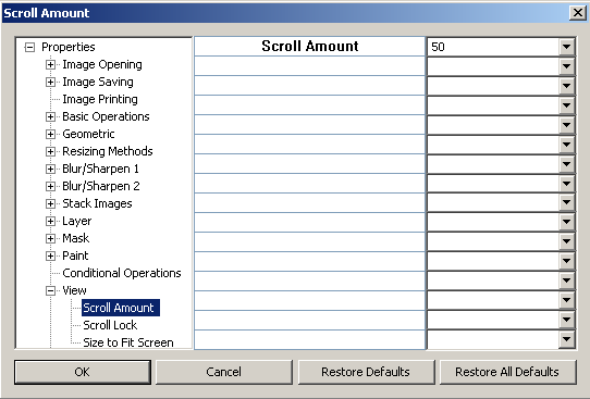
The Home key centers the image. Ctrl+Arrow (Alt+Ctrl+Arrow for 10X) keys actually shifts image within buffer (canvas) in top layer. When the image extends beyond the border of the buffer (canvas), it wraps around to the other side. That way nothing is lost if the image is translated back to its original position. Shift+Arrow (Alt+Shift+Arrow for 10X) keys translates image in bottom layer." Use F10 to dismiss a menu. Use Ctrl+Break key to abort operations that show a progress bar.
SAR treats RGBA as a color space. The alpha channel mixes the views of the RGB channels with either the window background color (black by default) or, if there is an image of equal dimensions in a second layer, the RGB channels of underlying image. The background color of the window can be changed with Q>View>Background Grey Level.
SAR reads and writes TARGA and PNG files with alpha channels. Except for FDIB files and files with alpha channels, reading an image file does not change the previous color space setting. However, when files with alpha channels are read, the color space is automatically converted to RGBA. Reading an FDIB file automatically converts the color space to the color space that existed when the file was saved.
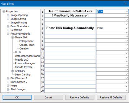
Because some operations are time consuming and use a large amount of RAM, it is usually necessary to use CommandLineSAR64.exe which requires a 64 bit version of the Windows Operating System. Look up the maximum number of threads for your CPU because you will use it. For example, for my Ryzen 7 2700X, the maximum number of threads is 16. Sorry, a GPU is not used calculations at this time.

To make an enlargement, select a neural net file (.net). Box2X.net, Box4X.net, Bicubic(-0.5)2X.net, Bicubic(-0.5)4X.net and Bicubic(-2)4X.net are the only such files packaged with SAR Image Processor v. 5.6. The "Box," etc. refer to the reduction methods used to train the neural nets. For most purposes, Box is best, but, Bicubic(-0.5) is most often used in contests therefore it is included for comparisons. "test.net" is the name of whatever file you create and train.
For best results, set line 3 to True. "8 Permutations" refers to the original, 90o rotation, 180o rotation, 270o rotation, horizontal flip, vertical flip, 90o rotation + horizontal flip, and 90o rotation + vertical flip.
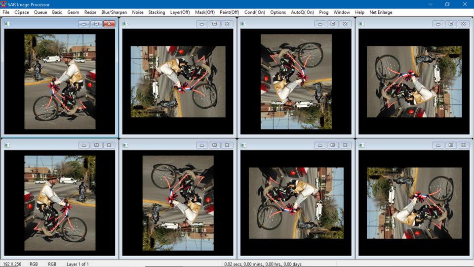
Ideally, an enlargement method should be invariant to these permutations, but neural nets are not and taking an average of results over these permutaions produces better results.
With the YCbCr Shortcut selected, only the Y channel of YCbCr color space is enlarged with the neural net.. The Cb and Cr channels are enlarged using Lanczos 3 interpolation.. With line 10 set to False, all channels are enlarged with the neural net. However, to produce the highest PSNR on the Y channel, set image to RGB color space, enlarge without the YCbCr shortcut, and then convert to YCbCr color space.
Important! This operation is greyed out in the menu unless you have an image loaded with the color space set to one that begins with Y, e.g., YCbCr. The reason for this is that only the Y channel is used in training.

First, select Create Net. Line 7 - This is the standard deviation of Gaussian distributed pseudorandom numbers used to initialize weights in the neural network. The best value depends on the activation function therefore use defaults. After clicking OK, another dialog box will appear.

Line 1 - The number of inputs can only be 8, 24, 48, 49 and 72. Only 48 is recommended; the others are for educational purposes. "48" represents a 7x7 image tile with the center pixel removed because its value is subtracted from the other pixel values. An optional "49" was included so you can prove to yourself that "48" is better. "72" consists of approximations to derivatives in a 7x7 tile, which produces slightly better results, but, requires more RAM.
Lines 3 and 4 - Only the default values are recommended because I determined them to be best.
Lines 5 - 20 - Important! The last layer with a nonzero number of neurons must have a number equal to 4 or 16 or else the program will crash. "4" represents a 2X enlargement and "16" represents a 4X enlargement. The neuron numbers of preceding layers should be multiples of 8 or 16 for reasons of speed. If the number of threads is 16 (make sure your CPU supports it) make those neuron numbers multiples of 16. I discovered that, with my MPL, it is not generally true that more layers or more neurons per layer, the better the results. The default numbers (the ones shown in the image) seem to be nearly optimal. After clicking OK, the neural net that you created will be saved to a file named "test.net" in the same directory as SARImageProcessor.exe.

Next, select Create Data Structure. Line 11 - Reduction Type can be set. After clicking OK, an Open File dialog box will appear. Select multiple image files, typically 100-200 0.25 megapixel images.
Links for training images include:
http://vllab.ucmerced.edu/wlai24/LapSRN/results/SR_training_datasets.zip
http://vllab.ucmerced.edu/wlai24/LapSRN/results/SR_testing_datasets.zip
Input and output tiles with the 8 aforementioned permutations will be created and stored in a file, "test.dat," in the same directory as SARImageProcessor.exe. The dimensions of the input and output tiles are determined from the previously created test.net, specifically the number of inputs and the number of neurons in the last layer. Thus, you can use the same test.dat on different test.net as long as those numbers coincide. You can add more image files with the operation, Add to Data Structure, and optionally mix reduction types.
Warning! The test.dat file can become very large very fast and you should not let it exceed half your RAM size, so check its size with File Explorer.
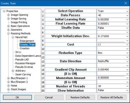
Next, select train. With the above settings, it takes my computer 14 hours to complete 40 passes through a 4 GB test.dat file. This is typically followed by another 40 passes with line 3 changed to 0.0001 to complete training, for a total of 28 hours. This may interfere with the simultaneous operation of some other programs. For example, I have trouble streaming Netflix with my Firefox browser while CommandLineSAR64.exe is running with 16 threads.
After training, you can save test.net under another name by selecting the opertation, Save Net As. Or, you can rename it using File Exlorer. From the enlargement dialog box, select either test.net or Other to use your neural net file.